Statistical Method 4 : Statistical Inference about Two Populations
두 모집단을 비교해보자
Difference in two means with known population variances
use z statistic
두 모평균의 차이는 \(\bar x_1-\bar x_2\)로 나타낼 수 있다. 이를 예시에 적용해보면, 두 브랜드의 치약이 동일하게 효과적인가? / 두 브랜드의 타이어가 다르게 닳는가? 등이 있다. CLT에 따라, x_1과 x_2의 표본의 크기가 모두 충분히 클 때(\(\geq 30\)), \(\bar x_1-\bar x_2\)도 정규분포를 따른다. \[\begin{aligned} \bar{x}_1 & \sim N\left(\mu_1, \frac{\sigma_1^2}{n_1}\right) \\ \bar{x}_2 & \sim N\left(\mu_2, \frac{\sigma_2^2}{n_2}\right) \\ \rightarrow \quad \bar{x}_1-\bar{x}_2 & \sim N\left(\mu_1-\mu_2, \frac{\sigma_1^2}{n_1}+\frac{\sigma_2^2}{n_2}\right) \end{aligned}\]
\(\bar x_1-\bar x_2\)의 평균(기댓값)은 \(\mu_1-\mu_2\), 분산은 \(\frac{\sigma_1^2}{n_1}+\frac{\sigma_2^2}{n_2}\)이다.
그러면 Z값으로 표준화시켜보자. \[z=\frac{\left(\bar{x}_1-\bar{x}_2\right)-\left(\mu_1-\mu_2\right)}{\sqrt{\frac{\sigma_1^2}{n_1}+\frac{\sigma_2^2}{n_2}}}\]
이 값을 검정하는 데에도 활용할 수 있다.
ex. Suppose we want to conduct a hypothesis test to determine whether the average annual wage for an auditing manager is different from the average annual wage of an advertising manager, where auditing managers are population 1 and advertising managers are population 2.
- A random sample of 34 auditing managers is taken.
- A similar random sample is taken of 32 advertising managers.
- The sample of auditing managers has a sample mean of $98,959 and a known population standard deviation of $12,709
- The sample of advertising managers has a sample mean of $95,433 and a known population standard deviation of $15,997
- Let α = 0.05, giving a z value of 1.96
H0의 값을 넣어서 계산해본다. \[z=\frac{\left(\bar{x}_1-\bar{x}_2\right)-\left(\mu_1-\mu_2\right)}{\sqrt{\frac{\sigma_1^2}{n_1}+\frac{\sigma_2^2}{n_2}}}=\frac{(98,959-95,433)-(0)}{\sqrt{\frac{12,709^2}{34}+\frac{15,997^2}{32}}} \approx 0.99\]
-> Since 0.99 < 1.96, we fail to reject the null hypothesis 1.96보다 작은 값이 나왔다. 즉 기각역에 포함이 되지 않으므로 H0은 유의수준 0.05 하에서 기각되지 않는다.
Confidence Interval
모평균 추정에서의 신뢰구간은 다음과 같았다. \(\bar{x}-z_{\alpha / 2} \frac{\sigma}{\sqrt{n}} \leq \mu \leq \bar{x}+z_{\alpha / 2} \frac{\sigma}{\sqrt{n}}\) 평균 + z값*표준편차다.
두 모평균의 추정도 상응하는 값을 넣으면 신뢰구간을 구할 수 있다. \[\left(\bar{x}_1-\bar{x}_2\right)-z_{\alpha / 2} \sqrt{\frac{\sigma_1^2}{n_1}+\frac{\sigma_2^2}{n_2}} \leq \mu_1-\mu_2 \leq\left(\bar{x}_1-\bar{x}_2\right)+z_{\alpha / 2} \sqrt{\frac{\sigma_1^2}{n_1}+\frac{\sigma_2^2}{n_2}}\]
Difference in two means with unknown population variances
use t statistic
samples are independent라는 가정이 필요하다. 해당 경우에서 우리는 모분산을 모르기 때문에, 두 모집단의 분산이 같은 경우(등분산성)와 다른 경우로 나누어 생각해보아야 한다.
1) 등분산 가정 \(\sigma_1^2=\sigma_2^2=\sigma^2\)
두 모집단의 분산이 같을 경우, 식을 다음과 같이 정리할 수 있다. \[z=\frac{\left(\bar{x}_1-\bar{x}_2\right)-\left(\mu_1-\mu_2\right)}{\sqrt{\frac{\sigma_1^2}{n_1}+\frac{\sigma_2^2}{n_2}}}=\frac{\left(\bar{x}_1-\bar{x}_2\right)-\left(\mu_1-\mu_2\right)}{\sigma \sqrt{\frac{1}{n_1}+\frac{1}{n_2}}}\]
그러면 우리는 추정해야 하는 모분산이 공통 모분산 \(\sigma^2\)으로 하나가 된다. 공통 모분산 \(\sigma^2\)의 추정량은 \(S^2_p\)이고, 그 추정값은 다음과 같다. 이렇게 계산된 표본분산은 합동표본분산(pooled sample variance)라고 한다. \[s_p^2=\frac{\left(n_1-1\right) s_1^2+\left(n_2-1\right) s_2^2}{n_1+n_2-2}\]
Note that \(\mathbb{E}\left[s_p^2\right]=\sigma^2\) Proof: \(\mathbb{E}\left[s_p^2\right]=\frac{\left(n_1-1\right) \mathbb{E}\left[s_1^2\right]+\left(n_2-1\right) \mathbb{E}\left[s_2^2\right]}{n_1+n_2-2}=\frac{\left(n_1-1\right) \sigma^2+\left(n_2-1\right) \sigma^2}{n_1+n_2-2}=\sigma^2\)
모집단의 분포가 독립이고 등분산 정규분포를 하는 경우 \(\bar x_1 - \bar x_2\)의 검정통계량인 \[t=\frac{\left(\bar{x}_1-\bar{x}_2\right)-\left(\mu_1-\mu_2\right)}{\sqrt {S^2_p(\frac{1}{n_1}+\frac{1}{n_2})}}\]
은 자유도가 n1+n2-2인 t분포를 따르게 된다.
2) 이분산 가정
두 모집단의 분산이 다르다고 가정하는 경우이다. 이 경우 s1과 s2를 구분해야 하기 때문에 다음과 같은 t값과 자유도의 공식이 나온다. 이 공식은 unpooled formula로 알려져 있다. \[t=\frac{\left(\bar{x}_1-\bar{x}_2\right)-\left(\mu_1-\mu_2\right)}{\sqrt{\frac{s_1^2}{n_1}+\frac{s_2^2}{n_2}}}, \quad \mathrm{df}=\frac{\left(\frac{s_1^2}{n_1}+\frac{s_2^2}{n_2}\right)^2}{\frac{\left(\frac{s_1^2}{n_1}\right)^2}{n_1-1}+\frac{\left(\frac{s_2^2}{n_2}\right)^2}{n_2-1}}\]
자유도의 소수점 이하는 버리고 정수부분만 사용한다.
(참고) 강의안에는 안 나왔는데, 신뢰구간은 다음과 같다. \[\bar{x}_1-\bar{x}_2 \pm t_{v, \alpha / 2} \sqrt{\frac{s_1^2}{n_1}+\frac{s_2^2}{n_2}}\]
Difference in two dependent populations
use t statistic
독립이 아닌 두 모집단의 차이이다. dependent samples, related samples를 다루기 위한 수단이다. Matched-pairs, correlated t test 로도 불린다. 예를 들면, 다이어트하기 전과 한 달 후의 몸무게처럼 동일한 개체에 대해 실험 전과 실험 후의 측정값의 차이를 추론할 수 있다. 두 모집단의 표본의 크기는 같아야 한다.
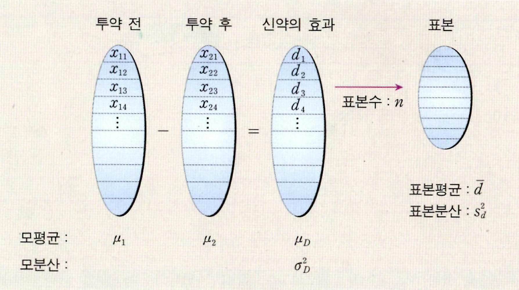 \[t=\frac{\bar{d}-D}{s_d / \sqrt{n}}, \quad \text { df }=n-1\]
\(\bar{d}=\frac{1}{n} \sum_{i=1}^n d_i\): 차이의 평균이다. \(s_d=\sqrt{\frac{\sum_{i=1}^n\left(d_i-\bar{d}\right)^2}{n-1}}\): 차이의 표준편차다. n: 짝의 개수 d_i: ith 짝의 차이 D: 모집단의 차이(\(\mu_D\))
예시 \[\begin{array}{|c|c|c|c|} \hline \text { COMPANY } & \text { YEAR 1 P/E } & \text { YEAR 2 P/E } & d \\ \hline 1 & 8.9 & 12.7 & -3.8 \\ \hline 2 & 38.1 & 45.4 & -7.3 \\ \hline 3 & 43.0 & 10.0 & 33.0 \\ \hline 4 & 34.0 & 27.2 & 6.8 \\ \hline 5 & 34.5 & 22.8 & 11.7 \\ \hline 6 & 15.2 & 24.1 & -8.9 \\ \hline 7 & 20.3 & 32.3 & -12.0 \\ \hline 8 & 19.9 & 40.1 & -20.2 \\ \hline 9 & 61.9 & 106.5 & -44.6 \\ \hline \end{array}\]
\[\begin{aligned} & H_0: D=0 \\ & H_a: D \neq 0 \end{aligned}\]
이렇게 데이터가 주어졌을 경우 각 짝 자료에 대해 차이(d)를 구하고, 그 평균과 분산도 직접 계산한다. \[n=9, \bar{d}=-5.033, s_d=21.599\] \[t=\frac{\bar{d}-D}{s_d / \sqrt{n}}=\frac{-5.033-0}{21.599 / \sqrt{9}}=-0.70\]
귀무가설을 두 모집단에 차이가 없다는 것으로 설정했기 때문에 D=0 이다.
−3.355 < − 0.70 < 3.355 이기 때문에 H0 기각 실패
신뢰구간은 다음과 같다. \[\bar{d}-t \frac{s_d}{\sqrt{n}} \leq D \leq \bar{d}+t \frac{s_d}{\sqrt{n}}, \quad \mathrm{df}=n-1\]
Difference in two population proportions
use z statistic
A집단의 불량률이 높은지, B집단의 불량률이 높은지 검정할 수 있다.
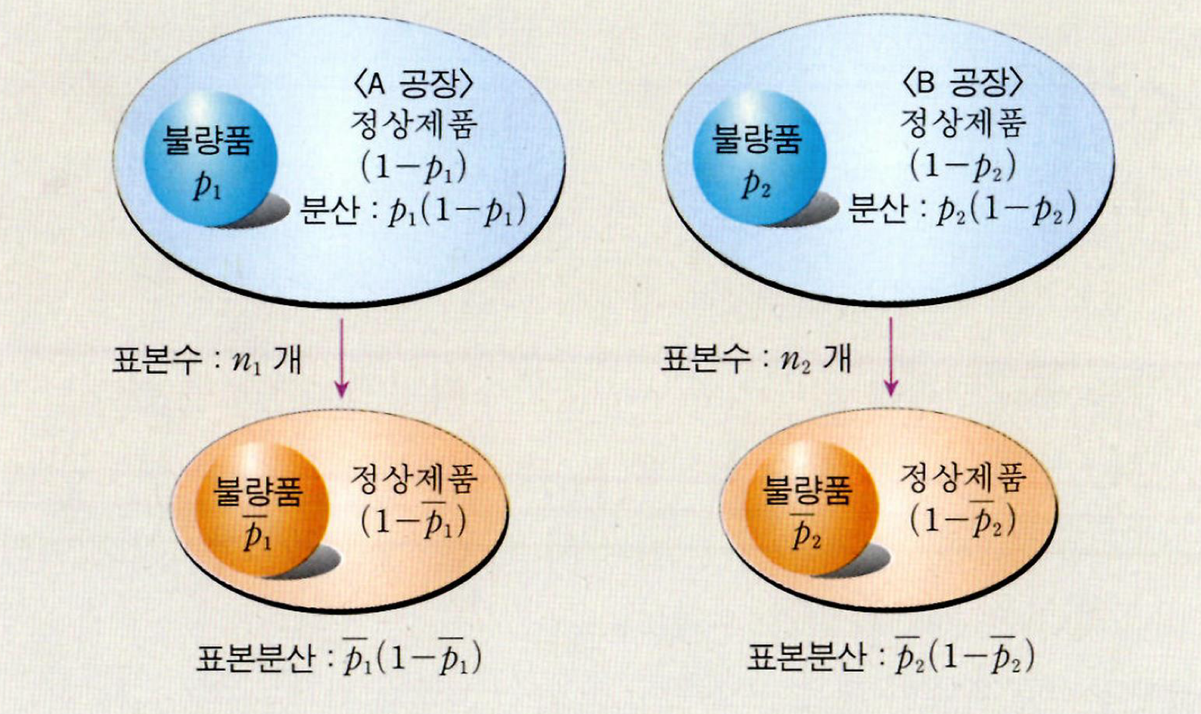 \(p_1, p_2\)는 모비율이다. \(q_1=1-p_1, q_2=1-p_2\)
CLT를 적용하려면, \(n_1 \hat{p}_1, n_1 \hat{q}_1, n_2 \hat{p}_2, n_2 \hat{q}_2>5\)여야 함을 잊지 말아야 한다. \[\begin{aligned} & \hat{p}_1 \sim N\left(p_1, \frac{p_1}{n_1}\right) \\ & \hat{p}_2 \sim N\left(p_2, \frac{p_2 q_2}{n_2}\right) \\ & \hat{p}_1-\hat{p}_2 \sim N\left(p_1-p_2, \frac{p_1 q_1}{n_1}+\frac{p_2 q_2}{n_2}\right) \end{aligned}\]
다른 검정통계량과 마찬가지로 평균과 표준편차를 활용해 계산한다. \[z=\frac{\left(\hat{p}_1-\hat{p}_2\right)-\left(p_1-p_2\right)}{\sqrt{\frac{p_1 q_1}{n_1}+\frac{p_2 q_2}{n_2}}}\]
이때 p1과 p2의 값을 추정해야 한다. \[z=\frac{\left(\hat{p}_1-\hat{p}_2\right)-\left(p_1-p_2\right)}{\sqrt{\bar{p} \bar{q}\left(\frac{1}{n_1}+\frac{1}{n_2}\right)}}\]
\(\bar{p}\) 값은 다음과 같이 추정할 수 있다. \[\bar{p}=\frac{x_1+x_2}{n_1+n_2}=\frac{n_1 \hat{p}_1+n_2 \hat{p}_2}{n_1+n_2} \text { and } \bar{q}=1-\bar{p}\]
Difference in two population variances
use F distribution
F분포란?
카이제곱분포는 한 정규모집단의 모분산을 추론하는 데에 사용되었다면, F분포는 두 정규모집단의 분산을 비교하는 데에 사용된다.
독립적인 카이제곱 변수 \(\chi_n^2\)와 \(\chi_m^2\)이 있을 때, \(X=\frac{\chi_n^2 / n}{\chi_m^2 / m}\)는 자유도가 n, m인 F분포를 따른다. \[X \sim F_{n, m}\]
- If \(X \sim t_n\) then \(X^2 \sim F_{1, n}\)
- \(F_{\alpha, n, m}\) is defined to be the value that satisfies \(\operatorname{Pr}\left(X>F_{\alpha, n, m}\right)=\alpha\) where \(\operatorname{Pr}\left(X>F_{\alpha, n, m}\right)=\alpha\)
- \[F_{1-\alpha, m, n}=\frac{1}{F_{\alpha, n, m}}\]
- \[P\left(X>F_{a, n, m}\right)=a\]
- \[P\left(1 / X<1 / F_{a, n, m}\right)=a\]
- \[P\left(1 / X>1 / F_{a, n, m}\right)=1-a\]
- \[1 / X=Y \sim F_{m, n}\]
- Thus \(F_{1-a, m, n}=1 / F_{a, n, m}\)
검정
- samples must be random and independent
- Each population must have a normal distribution
\(H_0: \sigma_1^2=\sigma_2^2\) test statistic: \(F=\frac{s_1^2}{s_2^2} \sim F_{n_1-1, n_2-1}\)
step1.
\(\begin{aligned} & H_0: \sigma_1^2=\sigma_2^2 \\ & H_a: \sigma_1^2 \neq \sigma_2^2 \end{aligned}\) (two-tailed)
step2. Since the population is normally distributed, the F test for the ratio of the variances can be used
step3. type I-error : \(\alpha=0.05\)
step4. Two-tailed test with \(\alpha / 2=0.025, \nu_1=n_1-1=9, \nu_2=n_2-1=11\) The critical F value for the upper tail is \(F_{0.025,9,11} = 3.59\)
- How to compute the lower tail value using the table?
- Use \(1 / F_{0.025,11,9} \approx 1 / 3.92=0.26\). Why?
- Remember the property: \(F_{1-\alpha, m, n}=\frac{1}{F_{\alpha, n, m}}\)
step5. 데이터에서 표본분산 구했다고 가정 \(F=\frac{s_1^2}{s_2^2}=\frac{0.11378}{0.02023}=5.62\)
The observed F value 5.62 is greater than the upper-tail critical value 3.59. Thus, reject the null hypothesis and conclude that the population variances are not equal.
참고: 연세대학교 손지용 교수님 통계방법론 강의안
<Excel, SPSS, R로 배우는 통계학 입문>