Statistical Method 1 : Sampling
다양한 샘플링 기법, 표본평균/분산, 표본평균의 평균/분산, CLT, FPC
Sampling
Population(모수): \(\mu\) = parameter 모집단을 표현 Sample(표본): \(\bar x\) = statistic 표본을 표현
Random Sampling: every unit of the population has the same probability of being selected into the sample (지향) Nonrandom Sampling: not every unit of the population ~ (지양. 통계방법론 적용에 부적절함)
Random Sampling Techniques
Simple Random Sampling
난수를 생성하여 임의로 뽑는다. 모수 N -> 표본 n
Stratified Sampling
Population is divided into non-overlapping subpopulations ex. age, gender, religion, etc. 집단을 구분하여 랜덤 샘플링 sample more closely match the population(error down) 집단 안에서는 동일하고 집단 밖에서는 배타적인 것이(겹치는게 없는) 이상적.
Proportionate stratified random sampling occurs when: the percentage of the sample taken from each stratum is proportionate to the percentage that each stratum is within the whole population 각 표본의 비율이 모집단에서의 비율과 같을 때 !!
Disproportionate different percentage
Systematic Sampling
Every kth item selected, sample size n, population size N, k=N/n ex. 순서대로 3의배수마다(?) 샘플 추출 (2,5,8..) 장점: convenient, 고르게(evenly) 분포된 샘플 단점: 데이터에 주기성이 있으면 bad
Cluster Sampling
Dividing populaiton into non-overlapping areas 아까랑 다르게, 하나의 집단 안에 다양한 사람들이 있고 그 집단이 다 비슷하게 생겨야 함. cluster should be a miniature of the population
장점: cluster가 명확하면 비용 등 효율적 단점: cluster의 요소가 비슷하면, simple random sampling보다 덜 효율적일 수 있음
Sampling Distribution
Sample Mean
표본평균: 평균의 추정. \(\bar{x}=\frac{1}{n} \sum_{i=1}^n x_i\) \[\mathbb{E}[\bar{x}]=\mu \& \mathbb{V}[\bar{x}]=\sigma^2 / n\]
\(E(X) = \mu\) \(V(X) = \sigma^2 = E(X^2)-E(X)^2\) \[E(\bar X) = \frac{1}{n}\sum^n_{i=1}E[X_i]=\frac{1}{n}\sum^n_{i=1}\mu=\mu\]
아래의 증명은 기억해두면 좋을 것 같다. \(\begin{aligned} & V(\bar{X})=V\left(\frac{1}{n} \sum_{i=1}^n X_i\right) \\ & =\frac{1}{n^2} V\left(\sum_{i=1}^n X_i\right) \\ & =\frac{1}{n^2} \sum_{i=1}^n V\left(X_i\right) \\ & =\frac{1}{n^2} \cdot n \cdot \sigma^2 \\ & =\frac{\sigma^2}{n} \end{aligned}\)
\(E(X) = \mu = \sum xf(x)\) \(Var(X) = E[(X-E(X))^2]\) 편차제곱의 평균
Sample Variance
\(s^2=\frac{1}{n-1} \sum_{i=1}^n\left(x_i-\bar{x}\right)^2\)
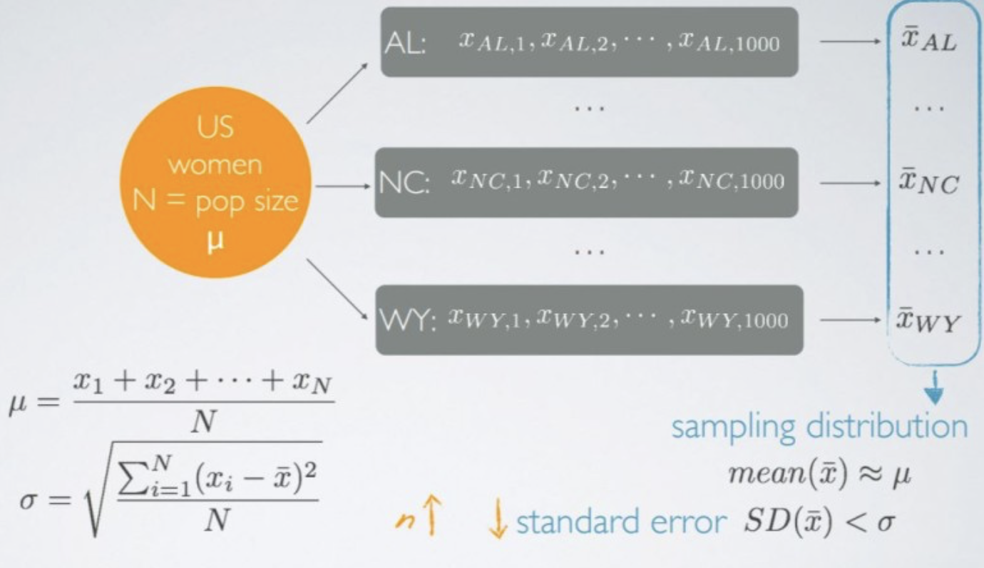 Duke university, 표본평균의 평균/분산
정리하자면, pop mean : \(\mu\) pop var : \(\sigma^2=E[(X-E(X))^2]=E(X^2)-E(X)^2\) sample mean : \(\bar x=\frac{1}{n} \sum_{i=1}^n x_i\) sample var : \(s^2=\frac{1}{n-1} \sum_{i=1}^n\left(x_i-\bar{x}\right)^2\) 표본평균의 평균 : \(E(\bar X)=\mu\) 표본평균의 분산: \(Var(\bar X)=\frac {\sigma^2}{n}\)
모평균을 모르기 때문에 sample mean으로 추정한다. 기댓값의 정의인 \(\sum xf(x)\)는 분포 f(x)를 알 때의 얘기!
자유도
“계산의 자유도”. 자유도 = 서로 독립적인 정보의 수. = 미지수(편의상!)-추정치 표본평균은 a+b+c/3으로 구한다. a,b,c 미지수 3개 = 자유도 3(n) 표본분산은 평균이 m일 때 (m-a)^2+(m-b)^2+(m-c)^2/2 a,b,c는 미지수, m은 a,b,c를 가지고 추정한 “추정치” 미지수에서 추정치 빼야 하기 때문에 3-1
왜 표본분산을 n-1로 나누는가 ?? = 자유도.
증명
\(s^2=\frac{1}{n} \sum_{i=1}^n\left(x_i-\bar{x}\right)^2\) 이라고 가정해보자. \[\begin{aligned} \mathbb{E}\left[s^2\right] & =\mathbb{E}\left[\frac{1}{n} \sum_{i=1}^n\left(x_i-\bar{x}\right)^2\right]=\mathbb{E}\left[\frac{1}{n} \sum_{i=1}^n\left(\left(x_i-\mu\right)-(\bar{x}-\mu)\right)^2\right] \\ & =\ldots=\mathbb{E}\left[\frac{1}{n} \sum_{i=1}^n\left(x_i-\mu\right)^2\right]-\mathbb{E}\left[(\bar{x}-\mu)^2\right]=\sigma^2-\mathbb{E}\left[(\bar{x}-\mu)^2\right]=\left(1-\frac{1}{n}\right) \sigma^2 \end{aligned}\]
즉, \(E(s^2) \neq \sigma^2\) 의 결과가 나와서 \(s^2\)이 unbiased estimator가 된다. => Thus, \(s^2=\frac{1}{n-1} \sum_{i=1}^n\left(x_i-\bar{x}\right)^2\)ensures that \(E(s^2)=\sigma^2\).
** \(s^2\)은 statistic, \(\sigma\)는 parameter.
표본평균의 분포 예시
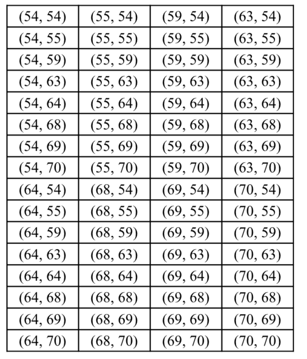
- 모집단을 54, 55, 59, 63, 64, 68, 69, 70 의 8개 숫자로 가정한다.
- n=2인 표본을 뽑는다.
- n=2인 모든 가능한 표본은 다음과 같이 나올 것이다.
 그리고 위의 표본들의 평균은 다음과 같이 나타낼 수 있다. (\(\bar X=\frac{1}{2}(X_1+X_2)\))
 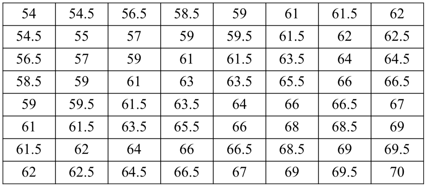 위의 표로 정리한 표본평균의 분포(오른쪽)은 모집단의 분포와 다른 것을 확인할 수 있다.
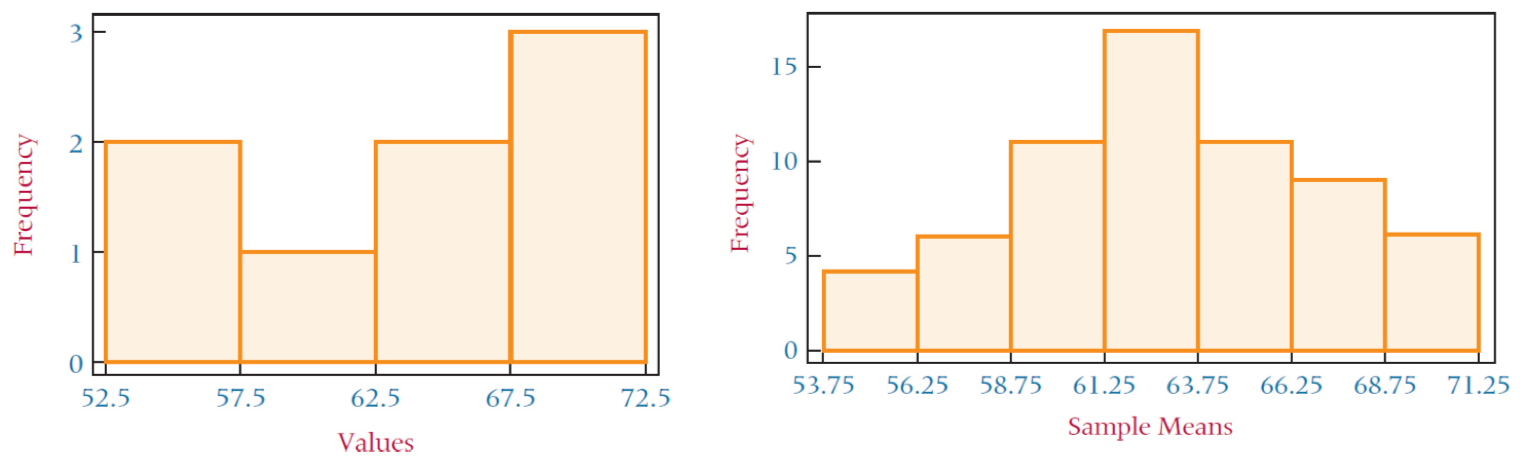
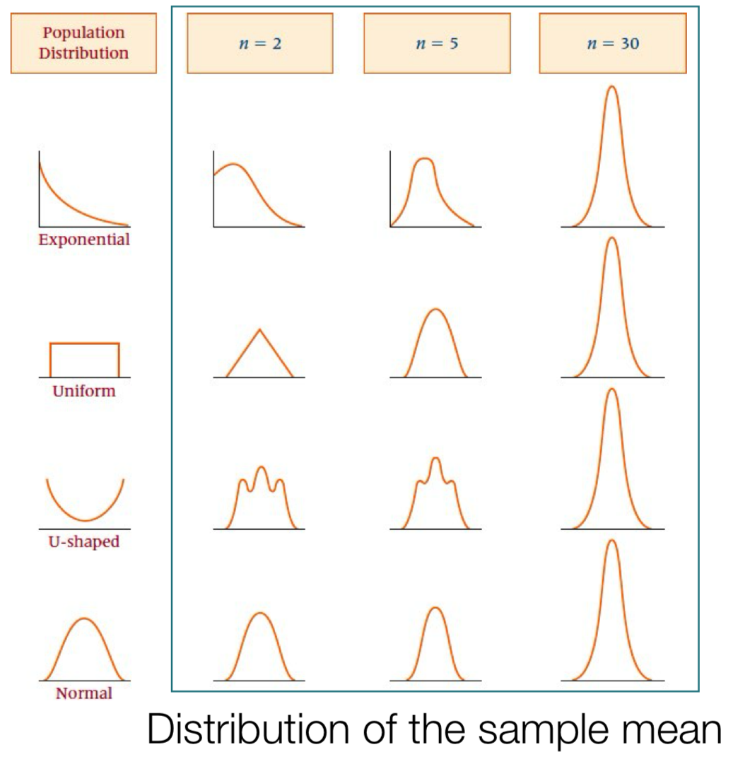
Central Limit Theorem (CLT)
+) i.i.d. : P(X_i=x_i, X_j=x_j)=P(X_i=x_i)P(X_j=x_j)
- \(X_1, ..., X_n\)이 평균 \(\mu\), 분산\(\sigma^2\)인 i.i.d.
- n이 충분히 클 때, \(\bar X \sim N(\mu, \frac {\sigma^2}{n})\)
- 모집단의 분포와 상관없이, 표본평균의 분포가 정규분포를 근사함.
- 보통 n>= 30.
- 모집단이 정규분포를 따를 경우, n의 크기와 상관없이 정규분포를 근사
표본평균의 평균: \(\mu_{\bar{x}}=\mu\) 표본평균의 표준편차: \(\sigma_{\bar{x}}=\frac{\sigma}{\sqrt{n}}\)
 n이 양의 무한대로 갈수록 표본평균의 분산은 0으로 수렴한다. 표본평균의 분산의 분모가 n이기 때문
- 표본의 크기가 충분히 크면 CLT가 적용됨
- 표본평균이 정규분포를 따름
- 각 수치를 측정하는 데에 z score이 쓰임 \(z=\frac{\bar{x}-\mu}{\sigma / \sqrt{n}}\sim N\left(0,1^2\right)\) 분모는 표본의 표준편차, 분자는 표본평균과 평균의 편차이다. 분포를 정리한 게시글(https://ese2o.github.io/stat/2024-02-29-stat3)에서도 소개했듯이, 이 z분포를 표준정규분포라고 부른다. ( : 정규분포를 표준화한 분포)
예시
Suppose the population mean amount of money spent per customer at a store is $125 and the population standard deviation is $30. If a random sample of 40 customers is taken, what is the probability that the sample mean expenditure is more than $133?
\(\mu = 125, \sigma=30, n=40\) \(P(\bar X >=133) ?\)
풀이 \(P(\bar X \geq 133)=P(z \geq \frac{133-125}{30/\sqrt{40}})\approx 1.69\) z분포표에 따르면, z=1.69의 확률은 0.4545 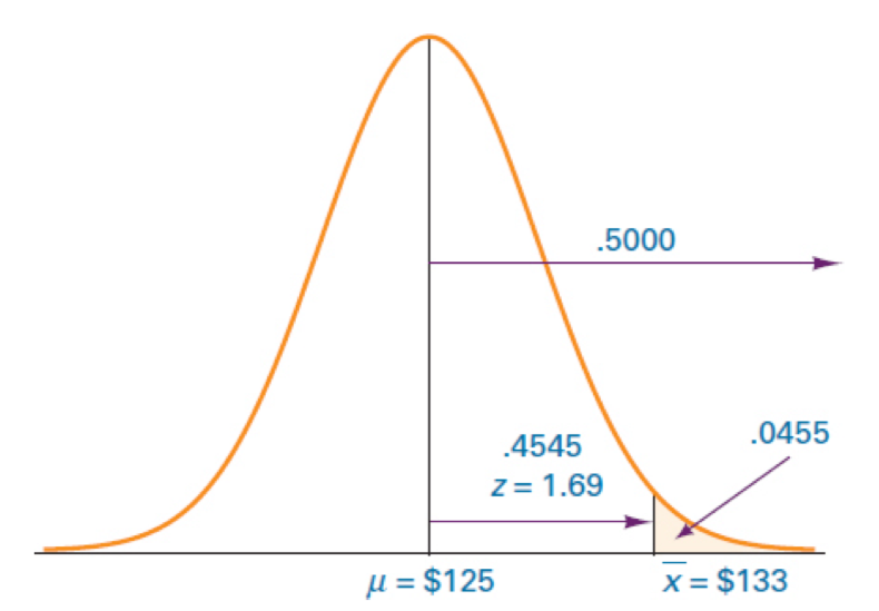
z가 1.69보다 클 확률이기 때문에 (위의 그림 참고) 0.5-0.4545 = 0.0455
Finite Population Correction (FPC)
지금까지는 모집단이 무한대이거나 충분히 클 때를 가정했음. 모집단이 유한하고 표본을 비복원추출할 경우, \(z=\frac{\bar{x}-\mu}{\frac{\sigma}{\sqrt{n}} \sqrt{\frac{N-n}{N-1}}}\) N은 모집단의 크기, n은 표본의 크기
\(n / N \geq 0.05\) 일 때 FPC 적용. N » n (훨씬 크다) 일수록 \(\sqrt{\frac{N-n}{N-1}}\)는 1로 수렴. FPC 참고자료
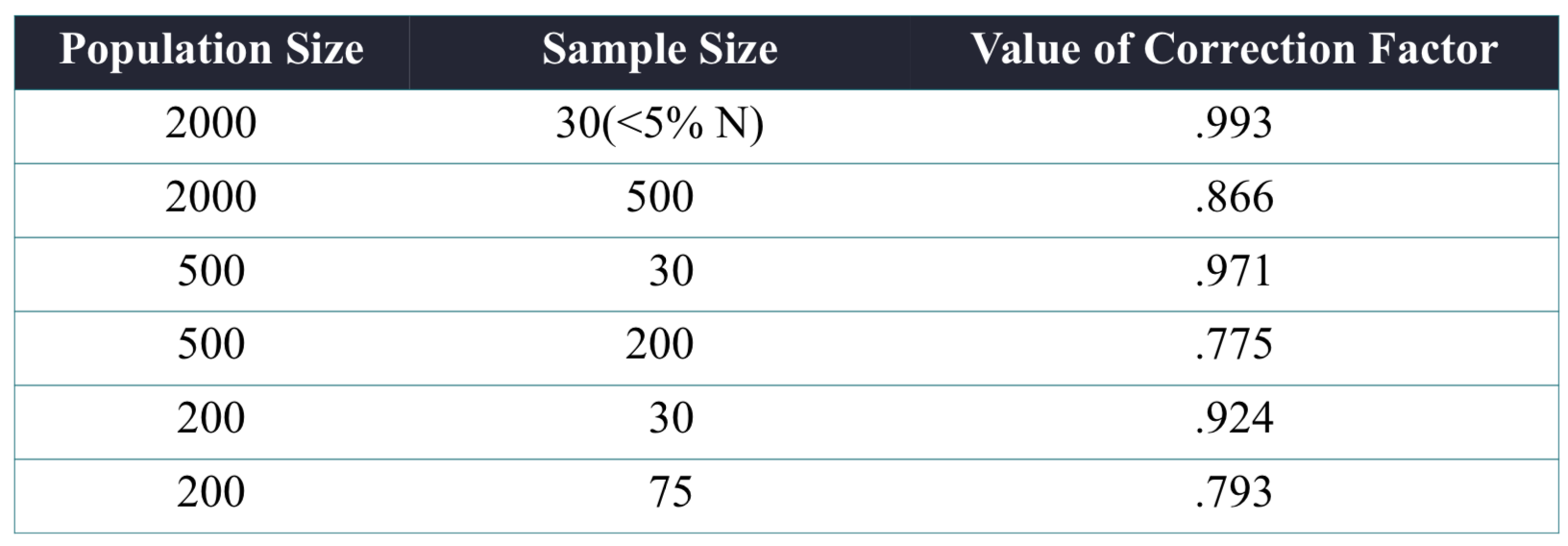 n=1일 때 FPC=1. \(0 \leq FPC \leq 1\)
Distribution of Sample Proportion
Sample Proportion
표본비율(\(\hat p\)): 모집단에서 추출한 표본들이 어떤 특징을 가지는 것들의 비율 computed by dividing the frequency with which a given characteristic occurs in the sample by the number of items in the sample
베르누이 시행에서 성공확률을 생각하면 된다.(이항분포를 따름)
\(\hat p=\frac {x}{n}\) n이 표본의 총 개수, x는 어떤 특징을 가지는 표본의 개수
\(X \sim B(n, p)\) \(E(X_i)=p\) \(\begin{aligned} \mathbb{E}[\hat{p}] & =\frac{1}{n} \mathbb{E}[x] \\ & =\frac{1}{n} \sum_{i=1}^n \mathbb{E}\left[x_i\right]=\frac{n p}{n}=p \\ \mathbb{V}[\hat{p}] & =\frac{\mathbb{V}(x)}{n^2}=\frac{n p q}{n^2}=\frac{p q}{n} \end{aligned}\)
- n이 충분히 클 때(\(np \geq 5, nq \geq 5\) where q=1-p) CLT에 따라 \(\hat p\)는 정규분포를 따른다. 표본비율의 평균은 p, 표본비율의 분산은 pq/n, 표본비율의 표준편차는 sqrt(pq/n)
정리하자면, \(\begin{aligned} & X \sim \operatorname{Binom}(n, p) \approx N(n p, n p q) \\ & \hat{p}=\frac{X}{n} \sim N\left(p, \frac{p q}{n}\right) \end{aligned}\)
표본비율이 X/n으로 구해지는데, X가 N(np,npq)를 따르고, 표본비율 p hat은 근사적으로 N(p, pq/n)을 따르게 되는 것이다.
예시
Suppose 60% of the electrical contractors in a region use a particular brand of wire. What is the probability of taking a random sample of size 120 from these electrical contractors and finding that 50% or less use that brand of wire?
p=0.6 n=120 \(P(\hat p \leq 0.5)\)?
풀이 np>5, nq>5 -> We can have CLT
\(z=\frac{\hat{p}-p}{\sqrt{p q / n}}\) \(z=\frac{0.5-0.6}{\sqrt{(0.6 \times 0.4) / 120}} \approx -2.24\)
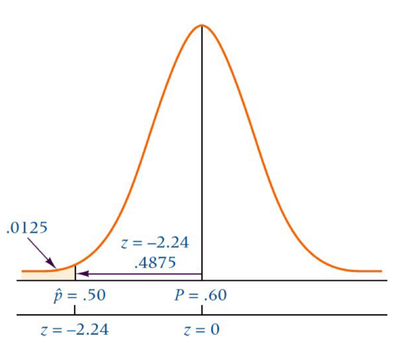 0.5-0.4875=0.0125
참고: 연세대학교 손지용 교수님 통계방법론 강의안
<Excel, SPSS, R로 배우는 통계학 입문>